Basic ideas and steps to build a neural network
In Note 1, we used numpy to build the simplest structural unit of the neural network: the perceptron. Note 2 will continue to learn how to build a neural network manually. We will learn how to use numpy to build a neural network with a single hidden layer. As the name implies, a single hidden layer is a neural network with only one hidden layer, or is it a two-layer network.
Continue to review the basic ideas and steps to build a neural network:
Define the network structure (specify the size of the output layer, hidden layer, and output layer)
Initialize model parameters
Loop operation: perform forward propagation/calculate loss/execute backward propagation/weight update
Define the network structure
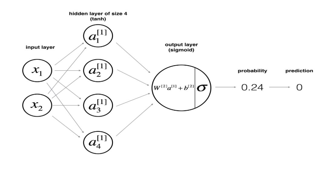
Suppose X is the input feature matrix of the neural network, and y is the label vector. Then the structure of the neural network with a single hidden layer is as follows:

The function of the network structure is defined as follows:
def layer_sizes(X, Y): n_x = X.shape[0] # size of input layer n_h = 4 # size of hidden layer n_y = Y.shape[0] # size of output layer return (n_x, n_h, n_y)
The size of the input layer and output layer are related to the shape of X and y respectively. The size of the hidden layer can be manually specified by us. Here we specify the size of the hidden layer as 4.
Initialize model parameters
Suppose W1 is the weight array from the input layer to the hidden layer, b1 is the bias array from the input layer to the hidden layer; W2 is the weight array from the hidden layer to the output layer, and b2 is the bias array from the hidden layer to the output layer. So we define the parameter initialization function as follows:
def initialize_parameters(n_x, n_h, n_y): W1 = np.random.randn(n_h, n_x)*0.01 b1 = np.zeros((n_h, 1)) W2 = np.random.randn(n_y, n_h)*0.01 b2 = np.zeros((n_y, 1)) assert (W1.shape == (n_h, n_x)) assert (b1.shape == (n_h, 1)) assert (W2.shape == (n_y, n_h) ) assert (b2.shape == (n_y, 1)) parameters = {"W1": W1, "b1": b1, "W2": W2, "b2": b2} return parameters
For the initialization of the weight, we use the module np.random.randn in numpy to generate random numbers, and the initialization of the bias uses the np.zero module. Encapsulate by setting a dictionary and return the result after initializing parameters.
Forward propagation
After the network structure is defined and the initialization parameters are completed, the training process of the neural network must be executed. The first step of training is to perform forward propagation calculations. Assume that the activation function of the hidden layer is the tanh function, and the activation function of the output layer is the sigmoid function. The forward propagation calculation is expressed as:

Define the forward propagation calculation function as:
def forward_propagation(X, parameters): # Retrieve each parameter from the dictionary "parameters" W1 = parameters['W1'] b1 = parameters['b1'] W2 = parameters['W2'] b2 = parameters['b2'] # Implement Forward Propagation to calculate A2 (probabilities) Z1 = np.dot(W1, X) + b1 A1 = np.tanh(Z1) Z2 = np.dot(W2, Z1) + b2 A2 = sigmoid(Z2) assert( A2.shape == (1, X.shape[1])) cache = {"Z1": Z1, "A1": A1, "Z2": Z2, "A2": A2} return A2, cache
Get the respective parameters from the parameter initialization result dictionary, then perform a forward propagation calculation, and save the result of the forward propagation calculation in the cache dictionary, where A2 is the result of the output layer after the sigmoid activation function is activated.
Calculate current training loss
After the forward propagation calculation is completed, we need to determine the loss between the output and the label value after the calculation is performed with the current parameters. Like note 1, the loss function is also selected as the cross-entropy loss:

Define the calculation loss function as:
def compute_cost(A2, Y, parameters): m = Y.shape[1] # number of example # Compute the cross-entropy cost logprobs = np.multiply(np.log(A2),Y) + np.multiply(np .log(1-A2), 1-Y) cost = -1/m * np.sum(logprobs) cost = np.squeeze(cost) # makes sure cost is the dimension we expect. assert(isinstance(cost, float )) return cost
Perform backpropagation
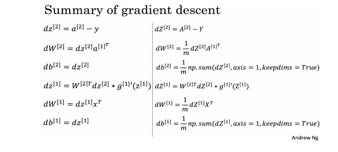
After the forward propagation and the current loss are determined, it is necessary to continue the back propagation process to adjust the weight. The gradient calculation of each parameter is involved, as shown in the following figure:

Define the back propagation function according to the above gradient calculation formula:
def backward_propagation(parameters, cache, X, Y): m = X.shape[1] # First, retrieve W1 and W2 from the dictionary "parameters". W1 = parameters['W1'] W2 = parameters['W2'] # Retrieve also A1 and A2 from dictionary "cache". A1 = cache['A1'] A2 = cache['A2'] # Backward propagation: calculate dW1, db1, dW2, db2. dZ2 = A2-Y dW2 = 1/ m * np.dot(dZ2, A1.T) db2 = 1/m * np.sum(dZ2, axis=1, keepdims=True) dZ1 = np.dot(W2.T, dZ2)*(1-np. power(A1, 2)) dW1 = 1/m * np.dot(dZ1, XT) db1 = 1/m * np.sum(dZ1, axis=1, keepdims=True) grads = {"dW1": dW1, "db1": db1, "dW2": dW2, "db2": db2} return grads
Put the derivation calculation result of each parameter into the dictionary grad and return it.
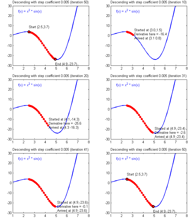
What needs to be mentioned here is the knowledge involved in numerical optimization. In machine learning, when the problem learned has a concrete form, machine learning will be formalized into an optimization problem. Whether it is gradient descent, stochastic gradient descent, Newton's method, quasi-Newton's method, or advanced optimization algorithms such as Adam, it takes time to master the mathematical principles.

Weight update
The last step of the iterative calculation is to update the weights according to the results of backpropagation. The update formula is as follows:

From this formula, the weight update function can be defined as:
def update_parameters(parameters, grads, learning_rate = 1.2): # Retrieve each parameter from the dictionary "parameters" W1 = parameters['W1'] b1 = parameters['b1'] W2 = parameters['W2'] b2 = parameters[ 'b2'] # Retrieve each gradient from the dictionary "grads" dW1 = grads['dW1'] db1 = grads['db1'] dW2 = grads['dW2'] db2 = grads['db2'] # Update rule for each parameter W1 -= dW1 * learning_rate b1 -= db1 * learning_rate W2 -= dW2 * learning_rate b2 -= db2 * learning_rate parameters = {"W1": W1, "b1": b1, "W2": W2, "b2" : b2} return parameters
In this way, the neural network training process of forward propagation-calculation loss-back propagation-weight update is even if the deployment is completed. Now, like note 1, in order to be more pythonic, we also combine the various modules to define a neural network model:
def nn_model(X, Y, n_h, num_iterations = 10000, print_cost=False): np.random.seed(3) n_x = layer_sizes(X, Y)[0] n_y = layer_sizes(X, Y)[2] # Initialize parameters, then retrieve W1, b1, W2, b2. Inputs: "n_x, n_h, n_y". Outputs = "W1, b1, W2, b2, parameters". parameters = initialize_parameters(n_x, n_h, n_y) W1 = parameters[ 'W1'] b1 = parameters['b1'] W2 = parameters['W2'] b2 = parameters['b2'] # Loop (gradient descent) for i in range(0, num_iterations): # Forward propagation. Inputs: "X, parameters". Outputs: "A2, cache". A2, cache = forward_propagation(X, parameters) # Cost function. Inputs: "A2, Y, parameters". Outputs: "cost". cost = compute_cost(A2, Y, parameters) # Backpropagation. Inputs: "parameters, cache, X, Y". Outputs: "grads". grads = backward_propagation(parameters, cache, X, Y) # Gradient descent parameter update. Inputs: "parameters, grads" . Outputs: "parameters". parameters = update_parameters(param eters, grads, learning_rate=1.2) # Print the cost every 1000 iterations if print_cost and i% 1000 == 0: print ("Cost after iteration %i: %f" %(i, cost)) return parameters
The above is the main content of this section. Use numpy to manually build a neural network with a single hidden layer. It is the best way to learn deep learning by writing from scratch, laying a firm foundation, and when the structure is proficient and the principles are thoroughly understood, and then contacting some mainstream deep learning frameworks.
General-purpose rectifiers belong to the most widely used category of rectifiers, and their classification is relative to those with special functions, such as fast, high-frequency, and so on.
Our universal rectifiers are of original quality, complete models, high visibility, affordable prices, and fast shipping!

Rectifiers,General Purpose Rectifiers,Rectifier Diode,General Purpose Rectifier Diodes
Changzhou Changyuan Electronic Co., Ltd. , https://www.cydiode.com
