Overfitting concepts and several regularization methods for solving overfitting problems
One of the most common problems encountered by data scientists in daily work and study is overfitting. Have you ever had such a model, it is excellent on the training set, but it is a mess on the test set. Have you ever had such an experience, when you participate in the modeling contest, from the running point of view your model should obviously top the list, but in the rankings announced by the side of the game, it is a great name, far away in hundreds of after that. If you have a similar experience, then this article is written specifically - it will tell you how to avoid overfitting to improve the performance of the model.

In this article, we will elaborate on the concept of overfitting and use several regularization methods for solving overfitting problems, supplemented by Python examples to further consolidate this knowledge. Note that this article assumes that the reader has some experience with neural networks and Keras.
What is regularization
Before delving into this topic, take a look at this picture:

Each time he talks about fitting, this picture will be pulled out from time to time as a "bite." As shown in the above figure, at the beginning, the model can not fit all the data points well, that is, it cannot reflect the data distribution. At this time, it is under-fitting. With the increase in the number of training, it slowly finds out the pattern of the data. It can reflect the data trend while fitting the data points as much as possible. At this time, it is a model with better performance. On this basis, if we continue to train, then the model will further tap into the details and noise in the training data. In order to fit all the data points "unscrupulously", it is overfitted.
In other words, from left to right, the complexity of the model gradually increases, and the prediction error on the training set gradually decreases, but its error rate on the test set presents a downward convex curve.
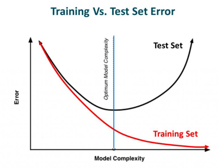
If you have built a neural network before, surely you have already learned this lesson: how complicated the network is, how easy it is to overfit. In order to make the model more generalized while fitting the data, we can use regularization to make some minor modifications to the learning algorithm to improve the overall performance of the model.
Regularization and overfitting
Over-fitting is closely related to the design of neural networks, so let's first look at an over-fit neural network:
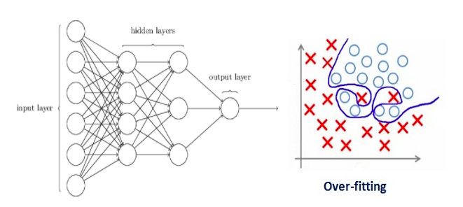
If you have read our zero-learning lessons before: understanding and coding neural networks (full version) from Python and R, or having a basic understanding of neural network regularization concepts, you should know that the lines with arrows in the figure above actually all carry The power is heavy, and the neuron is where input and output are stored. For the sake of fairness, that is, to prevent the network from flying too far in the direction of optimization, we also need to add a prior-regularization penalty term to punish the neuron's weighted matrix.
If we set the regularization coefficient to be large, resulting in the value of some weighting matrix is ​​almost zero - what we finally get is a simpler linear network, which is probably under-fitting.
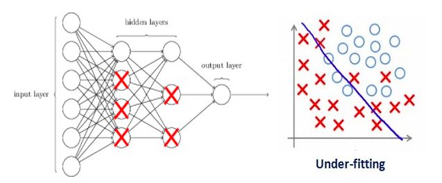
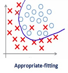
Therefore, this coefficient is not the bigger the better. We need to optimize the value of this regularization factor in order to get a well-fitting model, as shown in the figure below.
Regularization in deep learning
L2 and L1 regularization
L1 and L2 are the most common regularization methods. Their approach is to add a regularization term to the cost function.
Cost function = loss (eg binary cross entropy) + regularization term
Due to the addition of this regularization term, each weight is reduced, in other words, the complexity of the neural network is reduced, combining the idea of ​​how easy it is to have "how complicated the network is," theoretically That said, doing so is equal to preventing overfitting (Ocamham's razor rule).
Of course, this regularization term is not the same in L1 and L2.
For L2, its cost function can be expressed as:

Here λ is the regularization coefficient, which is a hyperparameter that can be optimized for better results. After derivation of the above equation, the coefficient before the weight w is 1−ηλ/m, because η, λ, and m are positive numbers, and 1−ηλ/m is less than 1, and the tendency of w is decreased, so the regularization of L2 is also Called weight attenuation.
For L1, its cost function can be expressed as:

Unlike L2, here we punish the absolute value of the weight w. After derivation of the above expression, we get an equation containing -sgn(w), which means that when w is positive, w decreases toward 0; when w is negative, w increases toward 0 . So the idea of ​​L1 is to put weight on 0, thereby reducing the complexity of the network.
Therefore, when we want to compress the model, the effect of L1 will be very good, but if it is simply to prevent over-fitting, L2 will still be used under normal circumstances. In Keras, we can directly call regularizers to regularize at any level.
Example: Using L2 regularized code in the full connection layer:
From keras Import regularizers
Model.add(Dense(64, input_dim=64,
Kernel_regularizer=regularizers.l2(0.01)
Note: Here 0.01 is the value of the regularization coefficient λ, we can further optimize it through grid search.
Dropout
Dropout is arguably the most interesting type of regularization method, and its effect is also very good, so it is one of the commonly used methods in the field of deep learning. To better explain it, let's first assume our neural network grows like this:
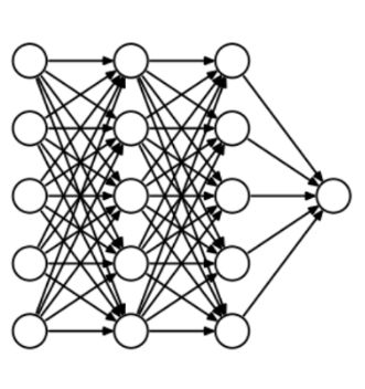
What did Dropout drop in the end? Let's take a look at the following picture: In each iteration, it randomly selects some neurons and "writes them" - "deleting" the neurons together with the corresponding input and output.
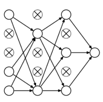
Compared to the modification of the cost function by L1 and L2, Dropout is more like a skill to train the network. As training progresses, the neural network will ignore some (hyperparameters, conventionally half) hidden/input neurons in each iteration, which leads to different outputs, some of which are correct and some are wrong.
This approach is somewhat similar to ensemble learning, it can capture more randomness. The ensemble learning classifier is usually better than a single classifier. Similarly, because the network fits the data distribution, most of the output of the model after Dropout is certainly correct, while the impact of noise data is only a small part, not The final result has a big impact.
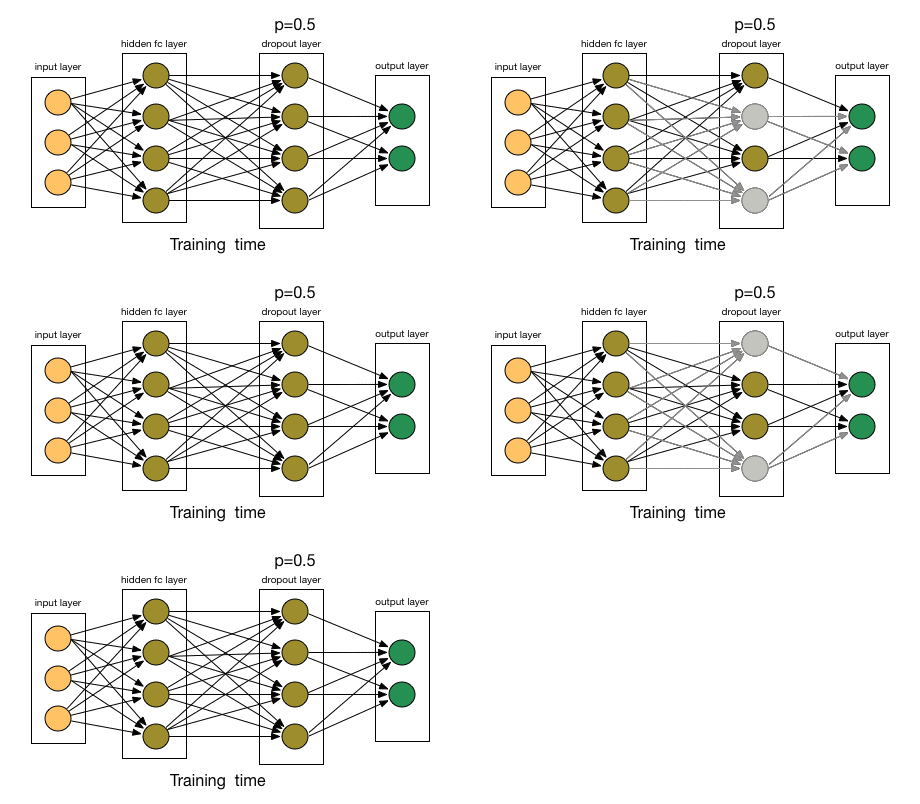
Due to these factors, we generally use Dropout when our neural network is larger and more random.
In Keras, we can use the keras core layer to achieve dropout. Here is its Python code:
From keras.layers.core importDropout
Model = Sequential([
Dense (output_dim=hidden1_num_units, input_dim=input_num_units, activation='relu'),
Dropout(0.25),
Dense (output_dim=output_num_units, input_dim=hidden5_num_units, activation='softmax'),
])
Note: Here we set 0.25 to the Dropout hyper-parameter (each time "deletion" 1/4), we can further optimize it through grid search.
Data enhancement
Since overfitting is the excessive capture of noise and detail in the dataset by the model, the easiest way to prevent overfitting is to increase the amount of training data. However, in machine learning tasks, increasing the amount of data is not easy to achieve, because the cost of collecting and marking data is too high.
Assume that we are dealing with some hand-written digital images. In order to expand the training set, we can use methods such as rotation, rollover, reduction/amplification, displacement, interception, addition of random noise, and addition of distortion. Here are some processed figures:

These are data enhancements. In a sense, the performance of the machine learning model is based on the amount of data, so the data enhancement can provide a huge improvement in the accuracy of model prediction. Sometimes it is a necessary skill to improve the model.
In Keras, we can use the ImageDataGenerator to perform all of these transformations. It provides a large list of parameters that can be used to preprocess training data. The following is the sample code that implements it:
From keras.preprocessing.image importImageDataGenerator
Datagen = ImageDataGenerator(horizontal flip=True)
Datagen.fit(train)
Early stop method
This is a cross validation strategy. Before training, we took a part of the training set as a verification set. As the training progressed, when the performance of the model on the verification set became worse, we immediately stopped the training manually. This method of early stop was the early stop method.
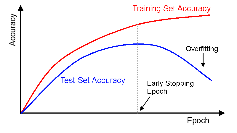
In the above figure, we should stop training at the dotted line, because after that, the model begins to overfit.
In Keras, we can stop the training ahead of time by calling the callbacks function. Here is its sample code:
From keras.callbacks importEarlyStopping
EarlyStopping(monitor='val_err', patience=5)
Here, monitor refers to the number of epochs that need to be monitored; val_err denotes a validation error.
Patience said that after 5 consecutive epoch models, the predictions did not improve further. According to the above figure, after the dashed line, the model will have a higher verification error for each epoch (lower verification accuracy). Therefore, after training five epochs in a row, it will stop training early.
Note: There is a situation when the model is trained on 5 epochs, its verification accuracy may increase, so we must be careful when selecting hyperparameters.
Investigating MNIST data with keras examples
Dataset: datahack.analyticsvidhya.com/contest/practice-problem-identify-the-digits/
After learning so many regularization methods, we must start practicing now. In this case, we used the digital identification data set of Analytics Vidhya.
We lead several basic libraries:
%pylab inline
Import numpy as np
Import pandas as pd
From scipy.misc import imread
From sklearn.metrics import accuracy_score
From matplotlib import pyplot
Import tensorflow as tf
Import keras
# Prevent potential randomness
Seed = 128
Rng = np.random.RandomState(seed)
Then load the data set:
Root_dir = os.path.abspath('/Users/shubhamjain/Downloads/AV/identify the digits/')
Data_dir = os.path.join(root_dir, 'data')
Sub_dir = os.path.join(root_dir, 'sub')
## only read training files
Train = pd.read_csv(os.path.join(data_dir, 'Train', 'train.csv'))
Train.head()
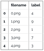
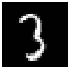
Check the image:
Img_name = rng.choice(train.filename)
Filepath = os.path.join(data_dir, 'Train', 'Images', 'train', img_name)
Img = imread(filepath, flatten=True)
Pylab.imshow(img, cmap='gray')
Pylab.axis('off')
Pylab.show()
# store images in a numpy array
Temp = []
For img_name in train.filename:
Image_path = os.path.join(data_dir, 'Train', 'Images', 'train', img_name)
Img = imread(image_path, flatten=True)
Img = img.astype('float32')
Temp.append(img)
X_train = np.stack(temp)
X_train /= 255.0
X_train = x_train.reshape(-1, 784).astype('float32')
Y_train = keras.utils.np_utils.to_categorical(train.label.values)
Create verification data set (7:3):
Split_size = int(x_train.shape[0]*0.7)
X_train, x_test = x_train[:split_size], x_train[split_size:]
Y_train, y_test = y_train[:split_size], y_train[split_size:]
Construct a simple neural network with 5 hidden layers, each containing 500 neurons:
# Import keras module
From keras.models importSequential
From keras.layers importDense
# define vars
Input_num_units = 784
Hidden1_num_units = 500
Hidden2_num_units = 500
Hidden3_num_units = 500
Hidden4_num_units = 500
Hidden5_num_units = 500
Output_num_units = 10
Epochs = 10
Batch_size = 128
Model = Sequential([
Dense (output_dim=hidden1_num_units, input_dim=input_num_units, activation='relu'),
Dense (output_dim=hidden2_num_units, input_dim=hidden1_num_units, activation='relu'),
Dense (output_dim=hidden3_num_units, input_dim=hidden2_num_units, activation='relu'),
Dense (output_dim=hidden4_num_units, input_dim=hidden3_num_units, activation='relu'),
Dense (output_dim=hidden5_num_units, input_dim=hidden4_num_units, activation='relu'),
Dense (output_dim=output_num_units, input_dim=hidden5_num_units, activation='softmax'),
])
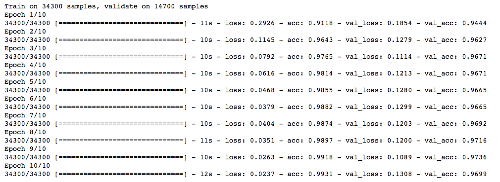
Run 10 epoch first, and quickly check the model performance:
Model.compile(loss='categorical_crossentropy', optimizer='adam', metrics=['accuracy'])
Trained_model_5d = model.fit(x_train, y_train, nb_epoch=epochs, batch_size=batch_size, validation_data=(x_test, y_test))
L2 regularization
From keras Import regularizers
Model = Sequential([
Dense (output_dim=hidden1_num_units, input_dim=input_num_units, activation='relu',
Kernel_regularizer=regularizers.l2(0.0001)),
Dense (output_dim=hidden2_num_units, input_dim=hidden1_num_units, activation='relu',
Kernel_regularizer=regularizers.l2(0.0001)),
Dense (output_dim=hidden3_num_units, input_dim=hidden2_num_units, activation='relu',
Kernel_regularizer=regularizers.l2(0.0001)),
Dense (output_dim=hidden4_num_units, input_dim=hidden3_num_units, activation='relu',
Kernel_regularizer=regularizers.l2(0.0001)),
Dense (output_dim=hidden5_num_units, input_dim=hidden4_num_units, activation='relu',
Kernel_regularizer=regularizers.l2(0.0001)),
Dense (output_dim=output_num_units, input_dim=hidden5_num_units, activation='softmax'),
])
Model.compile(loss='categorical_crossentropy', optimizer='adam', metrics=['accuracy'])
Trained_model_5d = model.fit(x_train, y_train, nb_epoch=epochs, batch_size=batch_size, validation_data=(x_test, y_test))
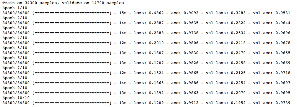
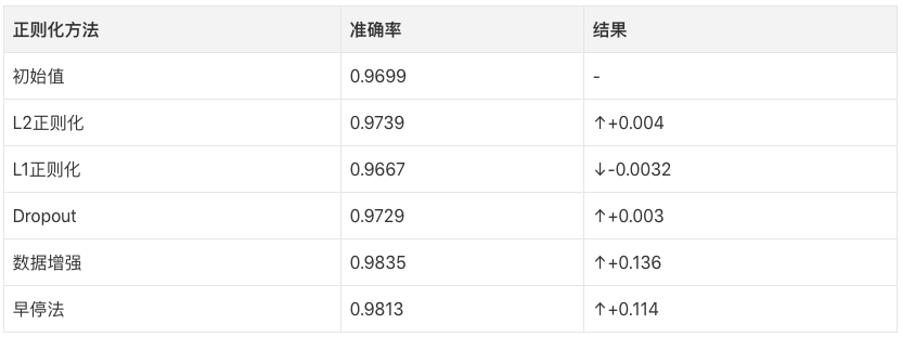
λ is equal to 0.0001, and the model prediction accuracy is higher!
L1 regularization
## l1
Model = Sequential([
Dense (output_dim=hidden1_num_units, input_dim=input_num_units, activation='relu',
Kernel_regularizer=regularizers.l1(0.0001)),
Dense (output_dim=hidden2_num_units, input_dim=hidden1_num_units, activation='relu',
Kernel_regularizer=regularizers.l1(0.0001)),
Dense (output_dim=hidden3_num_units, input_dim=hidden2_num_units, activation='relu',
Kernel_regularizer=regularizers.l1(0.0001)),
Dense (output_dim=hidden4_num_units, input_dim=hidden3_num_units, activation='relu',
Kernel_regularizer=regularizers.l1(0.0001)),
Dense (output_dim=hidden5_num_units, input_dim=hidden4_num_units, activation='relu',
Kernel_regularizer=regularizers.l1(0.0001)),
Dense (output_dim=output_num_units, input_dim=hidden5_num_units, activation='softmax'),
])
Model.compile(loss='categorical_crossentropy', optimizer='adam', metrics=['accuracy'])
Trained_model_5d = model.fit(x_train, y_train, nb_epoch=epochs, batch_size=batch_size, validation_data=(x_test, y_test))
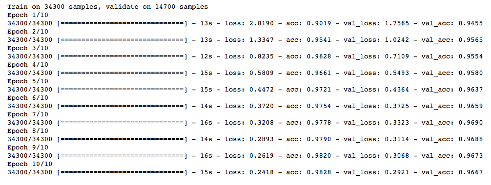
No improvement in the accuracy of the model, PASS!
Dropout
## dropout
From keras.layers.core importDropout
Model = Sequential([
Dense (output_dim=hidden1_num_units, input_dim=input_num_units, activation='relu'),
Dropout(0.25),
Dense (output_dim=hidden2_num_units, input_dim=hidden1_num_units, activation='relu'),
Dropout(0.25),
Dense (output_dim=hidden3_num_units, input_dim=hidden2_num_units, activation='relu'),
Dropout(0.25),
Dense (output_dim=hidden4_num_units, input_dim=hidden3_num_units, activation='relu'),
Dropout(0.25),
Dense (output_dim=hidden5_num_units, input_dim=hidden4_num_units, activation='relu'),
Dropout(0.25),
Dense (output_dim=output_num_units, input_dim=hidden5_num_units, activation='softmax'),
])
Model.compile(loss='categorical_crossentropy', optimizer='adam', metrics=['accuracy'])
Trained_model_5d = model.fit(x_train, y_train, nb_epoch=epochs, batch_size=batch_size, validation_data=(x_test, y_test))
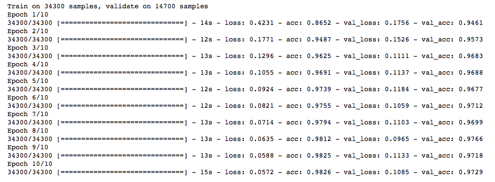
Also, the accuracy rate is higher than the beginning.
Data enhancement
From keras.preprocessing.image importImageDataGenerator
Datagen = ImageDataGenerator(zca_whitening=True)
# Download Data
Train = pd.read_csv(os.path.join(data_dir, 'Train', 'train.csv'))
Temp = []
For img_name in train.filename:
Image_path = os.path.join(data_dir, 'Train', 'Images', 'train', img_name)
Img = imread(image_path, flatten=True)
Img = img.astype('float32')
Temp.append(img)
X_train = np.stack(temp)
X_train = x_train.reshape(x_train.shape[0], 1, 28, 28)
X_train = X_train.astype('float32')
# Fit parameters from data - increase training data
Datagen.fit(X_train)
Here, we use zca_whitening, which highlights the outline of each number, as shown in the following figure:

## splitting
Y_train = keras.utils.np_utils.to_categorical(train.label.values)
Split_size = int(x_train.shape[0]*0.7)
X_train, x_test = X_train[:split_size], X_train[split_size:]
Y_train, y_test = y_train[:split_size], y_train[split_size:]
## reshaping
X_train=np.reshape(x_train,(x_train.shape[0],-1))/255
X_test=np.reshape(x_test,(x_test.shape[0],-1))/255
## structure using dropout
From keras.layers.core importDropout
Model = Sequential([
Dense (output_dim=hidden1_num_units, input_dim=input_num_units, activation='relu'),
Dropout(0.25),
Dense (output_dim=hidden2_num_units, input_dim=hidden1_num_units, activation='relu'),
Dropout(0.25),
Dense (output_dim=hidden3_num_units, input_dim=hidden2_num_units, activation='relu'),
Dropout(0.25),
Dense (output_dim=hidden4_num_units, input_dim=hidden3_num_units, activation='relu'),
Dropout(0.25),
Dense (output_dim=hidden5_num_units, input_dim=hidden4_num_units, activation='relu'),
Dropout(0.25),
Dense (output_dim=output_num_units, input_dim=hidden5_num_units, activation='softmax'),
])
Model.compile(loss='categorical_crossentropy', optimizer='adam', metrics=['accuracy'])
Trained_model_5d = model.fit(x_train, y_train, nb_epoch=epochs, batch_size=batch_size, validation_data=(x_test, y_test))
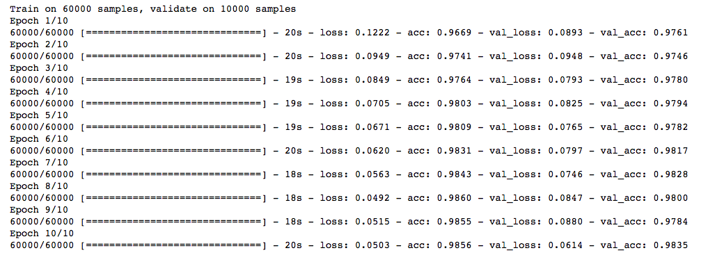
The promotion is very obvious!
Early stop method
From keras.callbacks importEarlyStopping
Model.compile(loss='categorical_crossentropy', optimizer='adam', metrics=['accuracy'])
Trained_model_5d = model.fit(x_train, y_train, nb_epoch=epochs, batch_size=batch_size, validation_data=(x_test, y_test)
, callbacks = [EarlyStopping(monitor='val_acc', patience=2)])

Compared with the above methods, the early stop method only stopped running five epochs, because the prediction accuracy rate did not increase. But if we increase the number of iterations, it should give better results.
Marine valve remote control device
Marine valve remote control device
Marine valve remote control device,valve remote control device,Marine valve remote control device price
Taizhou Jiabo Instrument Technology Co., Ltd. , https://www.taizhoujbcbyq.com
